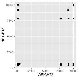
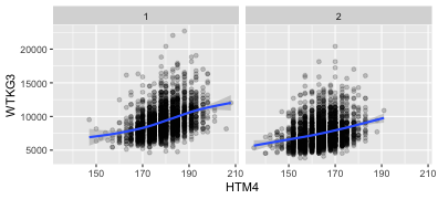
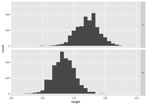
DS 202 - Working in teams: Sample solution for the test case

class: center, middle, inverse, title-slide

.title[
# DS 202 - Working in teams: Sample solution for the test case
]
.author[
### 
]

---

class: center, middle

# Solution to the test case

---

## A test case

The dataset `brfss_iowa.csv` (linked from website) contains 6227 records from the Behavioral Risk Factor Surveillance System (BRFSS) for Iowans.

> The Behavioral Risk Factor Surveillance System (BRFSS) is the nation's premier system of health-related telephone surveys that collect state data about U.S. residents regarding their health-related risk behaviors.

It is conducted annually by the Center for Disease Control and Prevention (CDC).

Codebook with detailed explanations of variables is [available here](https://www.cdc.gov/brfss/annual_data/2020/pdf/codebook20_llcp-v2-508.pdf).

---
class: inverse
## The Problem

0. Complete the following tasks and **write instructions / documentation** for a collaborator to be able to reproduce your findings.

1. Verify that there are 6227 cases (= number of interviews) in the data.

2. Verify that there are variables `WEIGHT2` and `HEIGHT3` in the data and read the description of the variables in the codebook.

3. How are height and weight related? Find correlations of weight and height by gender (`SEX`). How many values are the correlations based on for each gender?

2. Write a short report of your findings. Address potential problems in the data.

---

# A solution attempt

0. Setup

- this solution uses R v4.2.3 in RStudio (2023.06.2 Build 561). 
    - You need the R packages `tidyverse` and `rmarkdown` to run the solution
    - use the command `install.packages(c("tidyverse","rmarkdown"))` 
    in the R console to install the two packages

1. Navigate to https://github.com/ds202-at-ISU/materials

2. Download  the file [`test-case-solution.Rmd`](https://raw.githubusercontent.com/ds202-at-ISU/materials/master/01_collaborative-environment/test-case-solution.Rmd) in folder  `01_collaborative-environment`. Open the file in RStudio.

3. "Knit" the file (Click on the button in the menu).

---

## What is the relationship between height and weight?

Read the data:

```r
library(tidyverse)
iowa <- readr::read_csv("https://github.com/ds202-at-ISU/materials/raw/master/01_collaborative-environment/data/brfss_iowa.csv") 
```

```
## Warning: One or more parsing issues, call `problems()` on your data frame for details,
## e.g.:
##   dat <- vroom(...)
##   problems(dat)
```

```r
# the read_csv function from the readr package is faster than the standard read.csv
# but the output is a tibble (we'll come back to that)

iowa
```

```
## # A tibble: 6,227 × 330
##    X_STATE FMONTH IDATE    IMONTH IDAY  IYEAR DISPCODE     SEQNO  X_PSU CTELENUM
##      <dbl>  <dbl> <chr>    <chr>  <chr> <dbl>    <dbl>     <dbl>  <dbl>    <dbl>
##  1      19      7 07082015 07     08     2015     1200    2.02e9 2.02e9       NA
##  2      19      3 03212015 03     21     2015     1200    2.02e9 2.02e9       NA
##  3      19     10 01102016 01     10     2016     1200    2.02e9 2.02e9       NA
##  4      19      4 05092015 05     09     2015     1200    2.02e9 2.02e9       NA
##  5      19      5 06242015 06     24     2015     1200    2.02e9 2.02e9       NA
##  6      19      7 08032015 08     03     2015     1200    2.02e9 2.02e9       NA
##  7      19      7 08122015 08     12     2015     1200    2.02e9 2.02e9       NA
##  8      19      7 08102015 08     10     2015     1200    2.02e9 2.02e9       NA
##  9      19     10 11152015 11     15     2015     1200    2.02e9 2.02e9       NA
## 10      19      8 08132015 08     13     2015     1200    2.02e9 2.02e9       NA
## # ℹ 6,217 more rows
## # ℹ 320 more variables: PVTRESD1 <dbl>, COLGHOUS <lgl>, STATERES <dbl>,
## #   CELLFON3 <dbl>, LADULT <lgl>, NUMADULT <dbl>, NUMMEN <dbl>, NUMWOMEN <dbl>,
## #   CTELNUM1 <dbl>, CELLFON2 <dbl>, CADULT <dbl>, PVTRESD2 <dbl>,
## #   CCLGHOUS <dbl>, CSTATE <dbl>, LANDLINE <dbl>, HHADULT <dbl>, GENHLTH <dbl>,
## #   PHYSHLTH <dbl>, MENTHLTH <dbl>, POORHLTH <dbl>, HLTHPLN1 <dbl>,
## #   PERSDOC2 <dbl>, MEDCOST <dbl>, CHECKUP1 <dbl>, BPHIGH4 <dbl>, …
```

---

## Variables `HEIGHT3` and `WEIGHT2`

```r
iowa %>% select(HEIGHT3, WEIGHT2) %>% head()
```

```
## # A tibble: 6 × 2
##   HEIGHT3 WEIGHT2
##     <dbl>   <dbl>
## 1     511     191
## 2    7777     140
## 3     503     135
## 4     504     115
## 5      NA      NA
## 6     510     210
```

Variables are there ... but ... some data values look odd.

---

## Codebook excerpt

From the [codebook](https://www.cdc.gov/brfss/annual_data/2015/pdf/codebook15_llcp.pdf): HEIGHT3 and WEIGHT2 are the originally recorded variables.

Let's plot that ...

---

## Plot

Load the `ggplot2` package to plot weight versus height:

```r
iowa %>% 
  ggplot(aes(x = WEIGHT2, y = HEIGHT3)) + geom_point()
```

![](02_test-case-solution_files/figure-html/unnamed-chunk-3-1.png)

Height and weight should show a somewhat positive correlation. These clusters are an indication of the data coding.

---

## Next steps

Obviously, we need to spend some time cleaning these variables before we can make use of them.

We have a couple of choices:

1. We can buckle down and do that clean-up and then move on to the calculation.

2. We can take another look at the variables and investigate what `HTIN4`, `HTM4`, and `WTKG3` are ...

---

## Route 2

Let's take the second route first and draw a picture of height and weight in metric units:

```r
iowa %>% 
  ggplot(aes(x = HTM4, y = WTKG3)) + geom_point(alpha = 0.2) + 
  facet_grid(.~SEX) +
  geom_smooth()
```

![](02_test-case-solution_files/figure-html/unnamed-chunk-4-1.png)

These charts look much better! We see a general increase in weight as height increases. The variability in weight is huge, though. On average, women (`SEX = 2`) are shorter and lighter.

---

## Correlations of height and weight by gender

Based on variables `HTM4` and `WTKG3`

```r
iowa %>% 
  group_by(SEX) %>%
  summarize(
    n = n(),
    cor = cor(HTM4, WTKG3, use="pairwise.complete"),
    non_missing = sum(!is.na(HTM4) & !is.na(WTKG3)),
    non_missing_perc = non_missing/n*100
  )
```

```
## # A tibble: 2 × 5
##     SEX     n   cor non_missing non_missing_perc
##   <dbl> <int> <dbl>       <int>            <dbl>
## 1     1  2704 0.398        2589             95.7
## 2     2  3523 0.275        3051             86.6
```

---

## Route 1

This is a bit more work.

```r
# first of all, replace all missing values by NAs
iowa <- iowa %>% mutate(
  HEIGHT3 = replace(HEIGHT3, HEIGHT3 %in% c(7777,9999), NA),
  WEIGHT2 = replace(WEIGHT2, WEIGHT2 %in% c(7777,9999), NA)
)
```

Let's take on height first:

```r
iowa <- iowa %>% mutate(
  feet = HEIGHT3 %/% 100, # feet and inch only make sense for standard values,
  inch = HEIGHT3 %% 100,  # but we can calculated them for all
  height = ifelse(HEIGHT3 >= 9000, 
                  HEIGHT3 - 9000, # transform all metric values by subtracting 9000
                  feet *30.48 + 2.54*inch # add feet and inch converted to centimeter
                  )
)
```

---

## Now plot!

```r
iowa %>% filter(!is.na(height)) %>%
  ggplot(aes(x = height)) + geom_histogram(binwidth = 2.5) +
  facet_grid(SEX~.)
```

![](02_test-case-solution_files/figure-html/unnamed-chunk-8-1.png)

We get similar findings - for height at least: women are on average shorter than men.

---

## Route 1 (cont'd.)

do the same thing for weight as we did for height before: 1 pound is 0.454 kg

```r
iowa <- iowa %>% mutate(
  weight = ifelse(WEIGHT2 >= 9000, 
                  WEIGHT2 - 9000, # transform all metric values by subtracting 9000
                  WEIGHT2*.454 # 1 lbs = 0.454 kg
                  )
)
```

---

## Route 1

```r
iowa %>% 
  group_by(SEX) %>%
  summarize(
    n = n(),
    cor = cor(height, weight, use="pairwise.complete"),
    non_missing = sum(!is.na(height) & !is.na(weight)),
    non_missing_perc = non_missing/n*100
  )
```

```
## # A tibble: 2 × 5
##     SEX     n   cor non_missing non_missing_perc
##   <dbl> <int> <dbl>       <int>            <dbl>
## 1     1  2704 0.398        2589             95.7
## 2     2  3523 0.276        3051             86.6
```

---

## Recap

- Route 1 and 2 give identical solutions

- Read the codebook, visualize the data, even if the question does not ask for it.

```r
iowa %>% 
  group_by(SEX) %>%
  summarize(
    n = n(),
    cor = cor(HEIGHT3, WEIGHT2, use="pairwise.complete"),
    non_missing = sum(!is.na(HEIGHT3) & !is.na(WEIGHT2)),
    non_missing_perc = non_missing/n*100
  )
```

```
## # A tibble: 2 × 5
##     SEX     n   cor non_missing non_missing_perc
##   <dbl> <int> <dbl>       <int>            <dbl>
## 1     1  2704 0.424        2589             95.7
## 2     2  3523 0.357        3051             86.6
```

---

## Overview of the different height variables

```r
summary(iowa[,c("HEIGHT3", "HTIN4", "HTM4", "height")])
```

```
##     HEIGHT3           HTIN4            HTM4           height     
##  Min.   : 405.0   Min.   :53.00   Min.   :135.0   Min.   :134.6  
##  1st Qu.: 504.0   1st Qu.:64.00   1st Qu.:163.0   1st Qu.:162.6  
##  Median : 507.0   Median :67.00   Median :170.0   Median :170.2  
##  Mean   : 553.1   Mean   :67.12   Mean   :170.5   Mean   :170.5  
##  3rd Qu.: 510.0   3rd Qu.:70.00   3rd Qu.:178.0   3rd Qu.:177.8  
##  Max.   :9185.0   Max.   :82.00   Max.   :208.0   Max.   :208.3  
##  NA's   :232      NA's   :254     NA's   :232     NA's   :232
```

Why are there more missing values in `HTIN4`? - The official BRFSS data is missing any metric data in the variable `HTIN4`

---

## Recap

- this slide deck is rendered from an R Markdown document, located at [a github repo](https://github.com/Stat585-at-ISU/materials-2019/tree/master/01_collaborative-environment).

- code and text/documentation are interwoven: reproducible and self-documenting.

- extend or refine analyses by copying and modifying code blocks.

- disseminate your work by sharing the RMarkdown file

---

## Struggles can be informative

- we struggle with technology, the know how of the language ...

- ... others will too.

- remember those struggles when you write instructions for others to use your work