class: center, middle, inverse, title-slide .title[ # Intro to the tidyverse ] .author[ ### Will Ju ] --- # Data management in R: the tidyverse <img src="images/tidyverse.jpeg" alt="" width=500> --- # Outline - elements of data management: filtering, sorting, and aggregations - lots of examples --- # `tidyverse` `tidyverse` is a package bundling several other R packages: - `ggplot2`, `dplyr`, `tidyr`, `purrr`, ... - share common data representations and API, i.e. work well together - from the [tidyverse manifesto](https://tidyverse.tidyverse.org/articles/manifesto.html): 1. Reuse existing data structures. 2. Compose simple functions with the pipe. 3. Embrace functional programming. 4. Design for humans. - see https://github.com/hadley/tidyverse for more information --- # Common structure 1. all functions of the tidyverse have `data` as their first element ``` ggplot(data = fbi, aes(x = year, y = count)) + geom_point() filter(data = fbi, year >= 2017, state == "Iowa") ``` *i.e. work well with `%>%` operator* 2. *Most* functions return a data set. **The dimension of that data set is crucial, pay attention to it!** <br> <br> Important: do not use `$` notation for variables within these functions, e.g: --- ## The pipe operator `%>%` `f(x) %>% g(y)` is equivalent to `g(f(x), y)` i.e. the output of one function is used as input to the next function. This function can be the identity Consequences: - `x %>% f(y)` is the same as `f(x, y)` - statements of the form `k(h(g(f(x, y), z), u), v, w)` become `x %>% f(y) %>% g(z) %>% h(u) %>% k(v, w)` - read `%>%` as "then do" --- ## Using the pipe `%>%` ``` ggplot(data = filter(fbi, type=="homicide"), aes(x = year, y = count)) + geom_point() ``` becomes ``` library(tidyverse) fbi %>% filter(type=="homicide") %>% ggplot(aes(x = year, y = count)) + geom_point() ``` --- # `dplyr` There are a couple of primary `dplyr` *verbs*, representing distinct data analysis tasks: - `filter`: Select specified rows of a data frame, produce subsets - `mutate`: Add new or change existing columns of the data frame (as functions of existing columns) - `arrange`: Reorder the rows of a data frame - `select`: Select particular columns of a data frame - `summarize`: Create collapsed summaries of a data frame - `group_by`: Introduce structure to a data frame <br><br> RStudio cheat sheet for [dplyr](https://raw.githubusercontent.com/rstudio/cheatsheets/main/data-transformation.pdf) --- # `filter` .pull-left[ select a subset of the observations (horizontal selection): `filter (.data, ...)` specify constraints (as logical expression) to data in `...` all constraints are combined by logical and `&` ] .pull-right[  ] .footnote[Make sure to always call `library(dplyr)` before using `filter`] --- # `filter` Example From the `fbi` data, extract all burglaries in 2016: ```r library(classdata) library(dplyr) fbi %>% filter(type=="burglary", year==2016) %>% head() ``` ``` ## # A tibble: 6 × 8 ## state state_id state_abbr year population type count violent_crime ## <chr> <int> <chr> <int> <int> <chr> <int> <lgl> ## 1 Alabama 2 AL 2016 4860545 burglary 34045 FALSE ## 2 Alaska 1 AK 2016 741522 burglary 4053 FALSE ## 3 Arizona 5 AZ 2016 6908642 burglary 38216 FALSE ## 4 Arkansas 3 AR 2016 2988231 burglary 23814 FALSE ## 5 California 6 CA 2016 39296476 burglary 188304 FALSE ## 6 Colorado 7 CO 2016 5530105 burglary 23825 FALSE ``` --- # `mutate` .pull-left[ `mutate (.data, ...)` Introduce new variables into the data set or transform/update old variables multiple variables can be changed/introduced `mutate` works sequentially: variables introduced become available in following changes ] .pull-right[  ] --- # `mutate` Example Introduce a variable `Rate` into the `fbi` data: ```r fbi %>% mutate(rate = count/population*90000) %>% head() ``` ``` ## # A tibble: 6 × 9 ## state state_id state_abbr year population type count violent_crime rate ## <chr> <int> <chr> <int> <int> <chr> <int> <lgl> <dbl> ## 1 Alabama 2 AL 1983 3959000 homic… 364 TRUE 8.27 ## 2 Alabama 2 AL 1983 3959000 rape_… 931 TRUE 21.2 ## 3 Alabama 2 AL 1983 3959000 rape_… NA TRUE NA ## 4 Alabama 2 AL 1983 3959000 robbe… 3895 TRUE 88.5 ## 5 Alabama 2 AL 1983 3959000 aggra… 11281 TRUE 256. ## 6 Alabama 2 AL 1983 3959000 burgl… 42485 FALSE 966. ``` --- # `arrange` `arrange` sorts a data set by the values in one or more variables Successive variables break ties in previous ones `desc` stands for descending, otherwise rows are sorted from smallest to largest ```r fbi %>% arrange(desc(year), type, desc(count)) %>% head() ``` ``` ## # A tibble: 6 × 8 ## state state_id state_abbr year population type count violent_crime ## <chr> <int> <chr> <int> <int> <chr> <int> <lgl> ## 1 California 6 CA 2020 39368078 aggravat… 113646 TRUE ## 2 Texas 48 TX 2020 29360759 aggravat… 88810 TRUE ## 3 Florida 12 FL 2020 21733312 aggravat… 60871 TRUE ## 4 New York 38 NY 2020 19336776 aggravat… 46538 TRUE ## 5 Tennessee 47 TN 2020 6886834 aggravat… 37412 TRUE ## 6 Michigan 26 MI 2020 9966555 aggravat… 36384 TRUE ``` --- # `select` .pull-left[ Select specific variables of a data frame (vertical selection): `select (.data, ...)` specify all variables you want to keep Variables can be selected by index, e.g. `1:5`, by name (don't use quotes), or using a selector function, such as `starts_with` Negative selection also works, e.g. `-1` (not the first variable) ] .pull-right[  ] --- # `select` Example Select `type, count, state`, and `year` from the `fbi` data: ```r fbi %>% arrange(desc(year), type, desc(count)) %>% select(type, count, state, year) %>% head() ``` ``` ## # A tibble: 6 × 4 ## type count state year ## <chr> <int> <chr> <int> ## 1 aggravated_assault 113646 California 2020 ## 2 aggravated_assault 88810 Texas 2020 ## 3 aggravated_assault 60871 Florida 2020 ## 4 aggravated_assault 46538 New York 2020 ## 5 aggravated_assault 37412 Tennessee 2020 ## 6 aggravated_assault 36384 Michigan 2020 ``` --- class: inverse # Your turn Use the `fbiwide` data set from the `classdata` package Write out at least three different ways of selecting all variables describing incidences of different types of crimes --- # `summarize` .pull-left[ `summarize (.data, ...)` summarize observations into a (set of) one-number statistic(s): Creates a new dataset with 1 row and one column for each of the summary statistics ] .pull-right[  ] --- # `summarise` Example Calculate the mean and standard deviation of Crime rates in the `fbi` data ```r fbi %>% summarise(mean_rate = mean(count/population*90000, na.rm=TRUE), sd_rate = sd(count/population*90000, na.rm = TRUE)) ``` ``` ## # A tibble: 1 × 2 ## mean_rate sd_rate ## <dbl> <dbl> ## 1 467. 777. ``` --- # `summarize` and `group_by` .pull-left[ Power combo!  for each combination of group levels, create one row of a (set of) one-number statistic(s) The new dataset has one column for each of the summary statistics, and one row for each combination of grouping levels (multiplicative) ] .pull-right[ 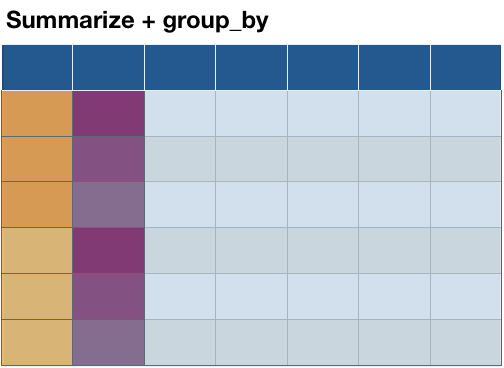 ] --- # `summarise` and `group_by` For each type of crime, calculate average crime rate and standard deviation. ```r fbi %>% group_by(type) %>% summarise(mean_rate = mean(count/population*90000, na.rm=TRUE), sd_rate = sd(count/population*90000, na.rm = TRUE)) ``` ``` ## # A tibble: 9 × 3 ## type mean_rate sd_rate ## <chr> <dbl> <dbl> ## 1 aggravated_assault 253. 146. ## 2 arson 24.1 15.2 ## 3 burglary 770. 389. ## 4 homicide 5.87 5.83 ## 5 larceny 2257. 749. ## 6 motor_vehicle_theft 317. 204. ## 7 rape_legacy 30.9 12.3 ## 8 rape_revised 40.1 17.6 ## 9 robbery 119. 126. ``` --- class: inverse, center, middle # Let's use these tools