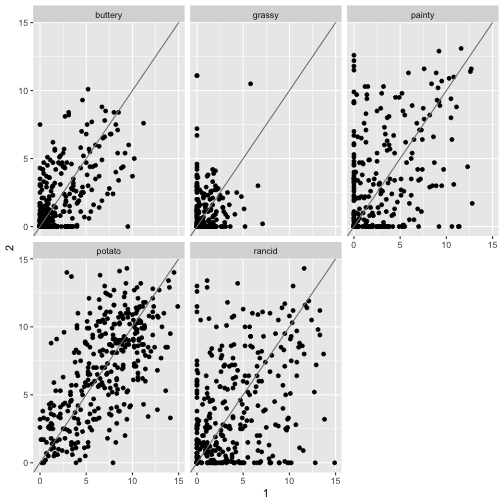
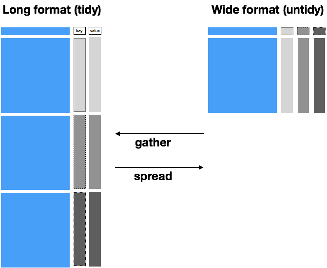
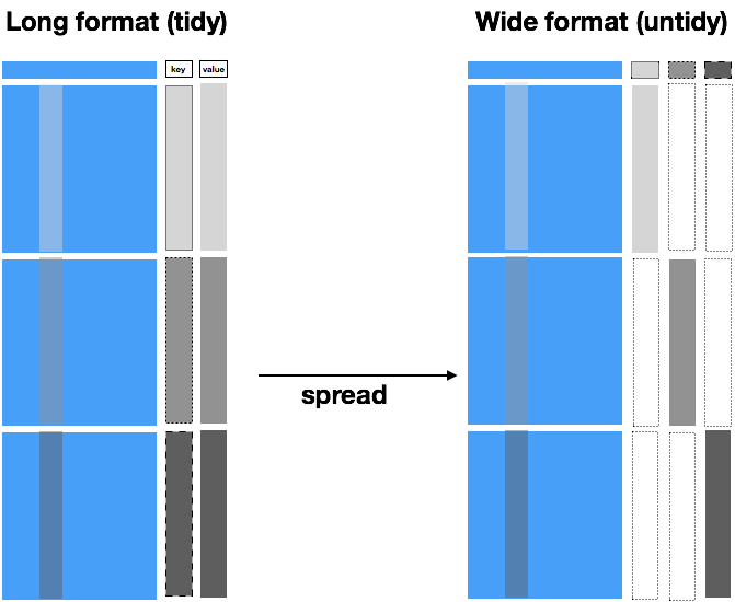
class: center, middle, inverse, title-slide .title[ # Reshaping data ] .author[ ### Will Ju ] --- class: middle, inverse, center # The `tidyr` package --- # What is tidy data? > Happy families are all alike; every unhappy family is unhappy in its own way.<br> Leo Tolstoy - `tidyr` vignette available as `vignette("tidy-data", package="tidyr")` - vignette is updated version of the [tidy data paper](https://www.jstatsoft.org/article/view/v059i10) with updated code --- # Outline - Different sources of messiness - Key-Value pairs - `tidyr`: `pivot_longer` and `pivot_wider` (former `gather` and `spread`) --- # Data often is in a spreadsheet format, but ... there's different ways of encoding the same information: Option #1 ``` ## name treatmenta treatmentb ## 1 John Smith NA 18 ## 2 Jane Doe 4 1 ## 3 Mary Johnson 6 7 ``` Option #2 ``` ## treatment John.Smith Jane.Doe Mary.Johnson ## 1 a NA 4 6 ## 2 b 18 1 7 ``` Neither #1 nor #2 are "clean" versions of the data: observed information is part of the data structure; some implicit information is assumed --- # Sources of Messiness 1. Column headers are values, not variable names.<br> e.g. *treatmenta, treatmentb* 2. Multiple variables are stored in one column.<br> e.g. *Fall 2015, Spring 2016* or *"1301 8th St SE, Orange City, Iowa 51041 (42.99755, -96.04149)", "2102 Durant, Harlan, Iowa 51537 (41.65672, -95.33780)"* 3. Multiple observational units are stored in the same table. 4. A single observational unit is stored in multiple tables. --- # Tidy data 1. Each variable forms one column. 2. Each observation forms one row. 3. Each type of observational unit forms a table. --- # Clean version of the example ``` ## treatment patient score ## 1 a John Smith NA ## 2 b John Smith 18 ## 3 a Jane Doe 4 ## 4 b Jane Doe 1 ## 5 a Mary Johnson 6 ## 6 b Mary Johnson 7 ``` - `treatment` and `patient` uniquely describe a single row in the dataset. - `treatment` and `patient` are **key variables**, - `score` is a **measurement variable** - this makes `treatment-patient` and `score` a **key-value pair** --- # Key-value pairs (KVP) **Key-Value pairs** (KVP) - also *attribute-value*, *field-value*, *name-value*: abstract data representation that allows a lot of flexibility One way of telling whether a data set is tidy is to check that all keys for a value are aligned in one row: | | | |:------------- |:------------- | | | | | <img src="images/kvp-unhappy.png" width=150> | <img src="images/kvp-happy.png" width=150> | |Untidy data | Tidy data | --- # Tidying data - Plan of attack Very few functions are needed for tidying data: - Messy (1): `tidyr` functions `pivot_longer` and `pivot_wider`. - `pivot_longer(data, cols, names_to = "name", values_to = "values")`: take multiple columns and collapse into key-value pairs - `pivot_wider (data, names_from=name, values_from=value)`: spread a key-value pair across multiple columns. - Messy (2): `tidyr` function `separate (data, col, into, sep = "[^[:alnum:]]+")`: separate one column into multiple columns - Messy (3): `dplyr` - some combination of the functions discussed previously - Messy (4): `dplyr` functionality `join` (and friends) to combine multiple data sets --- # French fries data ```r data(french_fries, package="reshape2") ``` - data from sensory experiment conducted at Iowa State University in 2004 - investigators were interested in comparing effects of three different fryer oils on taste of fries ```r french_fries %>% head() ``` ``` ## time treatment subject rep potato buttery grassy rancid painty ## 61 1 1 3 1 2.9 0.0 0.0 0.0 5.5 ## 25 1 1 3 2 14.0 0.0 0.0 1.1 0.0 ## 62 1 1 10 1 11.0 6.4 0.0 0.0 0.0 ## 26 1 1 10 2 9.9 5.9 2.9 2.2 0.0 ## 63 1 1 15 1 1.2 0.1 0.0 1.1 5.1 ## 27 1 1 15 2 8.8 3.0 3.6 1.5 2.3 ``` --- # Gather/Pivot to long ```r ffm <- french_fries %>% pivot_longer(cols = potato:painty, names_to = "scale", values_to = "score") ffm ``` ``` ## # A tibble: 3,480 × 6 ## time treatment subject rep scale score ## <fct> <fct> <fct> <dbl> <chr> <dbl> ## 1 1 1 3 1 potato 2.9 ## 2 1 1 3 1 buttery 0 ## 3 1 1 3 1 grassy 0 ## 4 1 1 3 1 rancid 0 ## 5 1 1 3 1 painty 5.5 ## 6 1 1 3 2 potato 14 ## 7 1 1 3 2 buttery 0 ## 8 1 1 3 2 grassy 0 ## 9 1 1 3 2 rancid 1.1 ## 10 1 1 3 2 painty 0 ## # ℹ 3,470 more rows ``` --- # Gather/Pivot to long <img src="images/gather-spread.png" height = 400> --- class: inverse # Your Turn Load the Avengers' data from FiveThirtyEight's survey into your work session: Data Description: [https://github.com/fivethirtyeight/data/tree/master/avengers](https://github.com/fivethirtyeight/data/tree/master/avengers) ```r av <- read.csv("https://raw.githubusercontent.com/fivethirtyeight/data/master/avengers/avengers.csv", stringsAsFactors = FALSE) ``` - Use the `select` function and the selector `starts_with` (read up on `?starts_with`) to select the name of the Avenger and all five death variables. Inspect the result with `head`. - Create a long form of the five death variables in the `av` data set using the function `pivot_longer`. Call the names `Time` and the values `Died`. Select `URL`, `Name.Alias`, `Time`, and `Died`, and save the result as `deaths`. Inspect the data set. - Create a (temporary) frequency breakdown of the variable `Died`. How can we interpret these numbers? --- # Pivot to wide ```r ffm %>% pivot_wider(names_from = rep, values_from = score) ``` ``` ## # A tibble: 1,740 × 6 ## time treatment subject scale `1` `2` ## <fct> <fct> <fct> <chr> <dbl> <dbl> ## 1 1 1 3 potato 2.9 14 ## 2 1 1 3 buttery 0 0 ## 3 1 1 3 grassy 0 0 ## 4 1 1 3 rancid 0 1.1 ## 5 1 1 3 painty 5.5 0 ## 6 1 1 10 potato 11 9.9 ## 7 1 1 10 buttery 6.4 5.9 ## 8 1 1 10 grassy 0 2.9 ## 9 1 1 10 rancid 0 2.2 ## 10 1 1 10 painty 0 0 ## # ℹ 1,730 more rows ``` ```r #ffm %>% spread(key = rep, value = score) ``` --- ```r ffm %>% pivot_wider( names_from = rep, values_from = score) %>% ggplot(aes(x = `1`, y = `2`)) + geom_point() + facet_wrap(~scale) + geom_abline(colour = "grey50") ``` <!-- --> --- class: inverse # Your turn For this your turn use the `french_fries` data from the `reshape2` package: `data("french_fries", package="reshape2")` - Use `pivot_longer` from the `tidyr` package to combine the different scales for assessing french fries into a single variable. Call the key-value pair "scale" and "score". - Use `pivot_wider` from the `tidyr` package to get a format in which you can directly compare values from week 1 to week 10. Plot a scatterplot of values in week 1 against week 10. Facet by treatment and scale, color by individuals and use different shapes for the replicates. Is there a pattern visible? --- class: inverse # Your turn For this your turn use the `fbiwide` data from the `classdata` package: `data("fbiwide", package="classdata")` - Use `pivot_longer` from the `tidyr` package to combine the variables for the different types of crimes into one variable. Call the key-value pair "Type" and "Incidences". Compute a crime rate - Only consider crime rates for Iowa and Minnesota. Use `pivot_wider` to create incidence columns for each of these states. Plot crimes in Iowa against crimes in Minnesota, colour by type of crime. Note: you need to exclude some variables. --- # `pivot_wider` works as inverse of `pivot_longer` ...  --- # Front part is not identical - not collapsible  --- # Where using `pivot_wider` is tricky - `pivot_wider` is the (almost) inverse operation of `pivot_longer` - when we use `pivot_longer` the key information is duplicated - when using `pivot_wider` we need to make sure that the information outside the key and value is identical for all levels (and combinations of levels) of the `key` variable. - If the info is not identical across levels, missing values are introduced into the new data set. --- # `pivot_wider` in the example ```r library(classdata) fbi %>% filter(year==2014, state_abbr %in% c("IA", "MN"), type=="burglary") ``` ``` ## # A tibble: 2 × 8 ## state state_id state_abbr year population type count violent_crime ## <chr> <int> <chr> <int> <int> <chr> <int> <lgl> ## 1 Iowa 16 IA 2014 3109481 burglary 14363 FALSE ## 2 Minnesota 27 MN 2014 5457125 burglary 20773 FALSE ``` Other state specific values don't allow spread to collapse the front part and introduce missing values: ```r fbi %>% filter(year==2014, state %in% c("Iowa", "Minnesota"), type=="burglary") %>% pivot_wider(names_from=state, values_from=count) ``` ``` ## # A tibble: 2 × 8 ## state_id state_abbr year population type violent_crime Iowa Minnesota ## <int> <chr> <int> <int> <chr> <lgl> <int> <int> ## 1 16 IA 2014 3109481 burglary FALSE 14363 NA ## 2 27 MN 2014 5457125 burglary FALSE NA 20773 ``` --- # fixing `pivot_wider` in the example Only select all relevant variables (or negative select all state-specific variables) to get the example to "work": ```r fbi %>% filter(year==2020, state_abbr %in% c("IA", "MN"), type=="burglary") %>% select(year, type, state, count) %>% pivot_wider(names_from=state, values_from=count) ``` ``` ## # A tibble: 1 × 4 ## year type Iowa Minnesota ## <int> <chr> <int> <int> ## 1 2020 burglary 11739 17370 ```