Polishing Plots

class: center, middle, inverse, title-slide

.title[
# Polishing Plots
]
.author[
### Will Ju
]

---

# Outline

- color choices

- themes

---
# `ggplot2` provides defaults ...

- but every aspect of the plot can be changed

- colors are controlled through **scales**

- **themes** control presentation of non-data elements

---

# Default continuous colour scheme

```r
library(tidyverse)
p1 <- mpg %>% filter(year == 2008) %>%
  ggplot(aes(x = cty, y = hwy, colour = cyl)) +
  geom_point()
```

```r
p1 + scale_colour_continuous()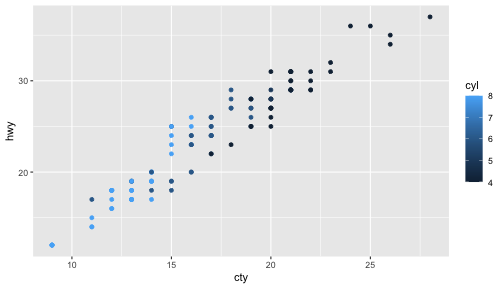
```

![](01_polishing-plots_files/figure-html/unnamed-chunk-2-1.png)

---

# Default discrete colour scheme

```r
p2 <- mpg %>% filter(year == 2008) %>%
  ggplot(aes(x = cty, y = hwy, colour = factor(cyl))) +
  geom_point()
```

```r
p2 + scale_colour_discrete()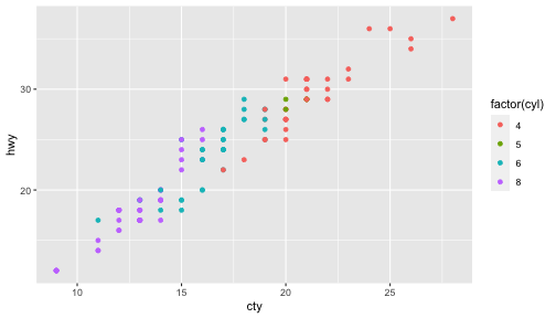
```

![](01_polishing-plots_files/figure-html/unnamed-chunk-4-1.png)

---

# Color Scales

- Colors are controlled through scales
`scale_colour_discrete` (`scale_colour_hue`) and `scale_colour_continuous` (`scale_colour_gradient`) are the default choices for factor variables and numeric variables

- we can change parameters of the default scale, or we can change
the scale function

---

# Colour gradients

`scale_colour_gradient (..., low = "#132B43", high = "#56B1F7", space = "Lab", na.value = "grey50", guide = “colourbar")`

- colors can be specified by hex code, name or through rgb()

- gradient goes from low to high - that should match the interpretation of the mapped variable

---

# Colour gradients - divergent scheme

`scale_colour_gradient2(..., low = muted("red"), mid = "white",  
high = muted("blue"), midpoint = 0, space = "Lab", na.value = "grey50",  guide = "colourbar")`

- midpoint is value of the ‘neutral’ color gradient2 is a divergent color scheme

- best matches a variable that goes from large negative to zero to large positive (or below mean, above mean)

---

```r
mean(mtcars$mpg)
```

```
## [1] 20.09062
```

```r
mtcars %>% 
  ggplot(aes(x = mpg, colour=mpg, y = 1)) + 
  geom_vline(xintercept=20) +
  geom_point(size = 5) +
  scale_colour_gradient2(midpoint = 20)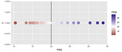 
```

![](01_polishing-plots_files/figure-html/unnamed-chunk-5-1.png)

---

# Discrete color schemes

`scale_color_hue (..., h = c(0, 360) + 15, c = 100, l = 65, h.start = 0, direction = 1, na.value = "grey50")`

- uses hue, chroma and luminance (=value)

- each level of a variable is assigned a different level of h

---

# Discrete color schemes - Brewer

`scale_colour_brewer(..., type = "seq", palette = 1, direction = 1)`

- brewer schemes are defined in RColorBrewer (Neuwirth, 2014) palettes can be specified by name or index

- see also http://colorbrewer2.org/ (Brewer et al 2002)

```r
mtcars %>% 
  ggplot(aes(x = mpg, colour=factor(cyl), y = 1)) + 
  geom_point(size = 5) +
  scale_color_brewer(type="qual")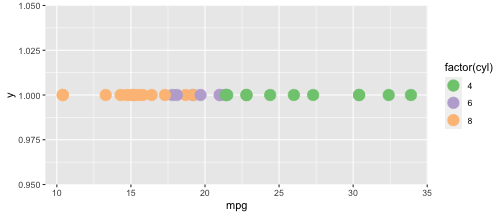
```

![](01_polishing-plots_files/figure-html/unnamed-chunk-6-1.png)
---

# All brewer schemes

```r
library(RColorBrewer)
display.brewer.all()
```

![](01_polishing-plots_files/figure-html/unnamed-chunk-7-1.png)

---

# Color and Fill

- Area geoms (barcharts, histograms, polygons) use `fill` to map values to the fill color

- only discrete color scales can be used:  `scale_fill_hue`, `scale_fill_brewer`, `scale_fill_grey`, ...

- most general: `scale_fill_manual (..., values)` 
values is a vector of color values. At least as many colors as levels in the variable have to be listed

---

# Themes

- Themes allow to control every aspect of non-data related aspects of a plot

- Several pre-defined themes: `theme_grey` (default), `theme_bw`, `theme_light`, `theme_dark`

- Use `theme_set` if you want it to apply a theme to every future plot, e.g. `theme_set(theme_bw())`

- `ggthemes` package defines additional themes: 
`library(help = "ggthemes")` lists all themes

---

# Example

```r
p <- mpg %>% ggplot(aes(x = displ, y =  cty, colour= factor(class))) + geom_point()
```

.pull-left[

```r
p + theme_grey()
```

![](01_polishing-plots_files/figure-html/unnamed-chunk-9-1.png)
]

.pull-right[

```r
p + theme_bw()
```

![](01_polishing-plots_files/figure-html/unnamed-chunk-10-1.png)
]

---

# Example - more themes

```r
p <- mtcars %>% ggplot(aes(x = wt, y =  mpg, colour= factor(cyl))) + geom_point()
```

.pull-left[

```r
p + theme_light()
```

![](01_polishing-plots_files/figure-html/unnamed-chunk-12-1.png)
]

.pull-right[

```r
p + theme_dark()
```

![](01_polishing-plots_files/figure-html/unnamed-chunk-13-1.png)
]

---

# More themes

```r
library(ggthemes)
```

.pull-left[

```r
p + theme_excel() 
```

![](01_polishing-plots_files/figure-html/unnamed-chunk-15-1.png)
]
.pull-right[

```r
p + theme_fivethirtyeight()
```

![](01_polishing-plots_files/figure-html/unnamed-chunk-16-1.png)
]

---

# Making charts readable

.pull-left[

```r
p + theme_light(base_size=18) 
```

![](01_polishing-plots_files/figure-html/unnamed-chunk-17-1.png)
]
.pull-right[

```r
p + theme_light(base_size=24)
```

![](01_polishing-plots_files/figure-html/unnamed-chunk-18-1.png)
]

---

# Elements

- You can also make your own theme, or modify an existing.

- Themes are made up of elements which can be one of:
`element_line`,  `element_text`, `element_rect`,
`element_blank`

- Gives you a lot of control over plot appearance.

---

# Elements of themes

- Axis:  
  `axis.line`, `axis.text.x`, `axis.text.y`, `axis.ticks`, `axis.title.x`, `axis.title.y`

- Legend:  
`legend.background`, `legend.key`, `legend.text`, `legend.title`

- Panel:  
`panel.background`, `panel.border`, `panel.grid.major`, `panel.grid.minor`

- Strip (facetting):  
`strip.background`, `strip.text.x`, `strip.text.y`

for a complete overview see `?theme`

---

# Changing elements manually

- to change an element add the theme function and specify inside:

- example:

```r
mpg %>% ggplot(aes(x = manufacturer)) + geom_bar() +
  theme(axis.text.x = element_text(angle=90, vjust=0.5, hjust=1))
```

![](01_polishing-plots_files/figure-html/unnamed-chunk-19-1.png)